The Diffuser plug-in is divided into several modules which correspond to different stages of the surface reconstruction pipeline:
• Preprocessing
• Distance Field
• Volumetric Diffusion
• Surface Reconstruction
• Extras
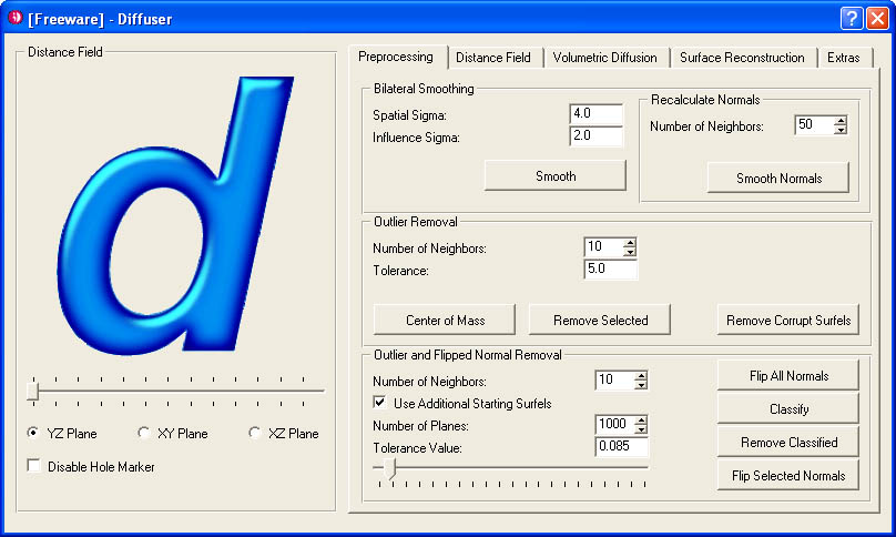
The preprocessing module contains a bilateral denoising filter and two outlier removal tools. The bilateral denoiser is set up with two parameters for the Gaussian filter: Spatial Sigma and Influence Sigma. When the normals of a given input model are very disturbed the algorithm does not always generate a satisfying point cloud as result. One possible solution is to recalculate the normals, but this introduces additional smoothing. The outlier removal with center of mass calculation can be applied to identify outliers using only their spatial information. The Tolerance value is multiplied with the averaging distance between the surfels and indicates the maximal distance allowed for the center of mass point. The surfels are selected when using the Center of Mass button - the user has to confirm with the Remove Selected button to definitely remove the surfels. This allows adjusting the parameters until a desired result is achieved. The Remove Corrupt Surfels function deletes surfels with an undefined normal, undefined tangent axes or a radius of zero. The third tool can be used to classify and remove outliers and surfels with flipped normals. The Tolerance Value can either be adjusted using the slider or by editing the value in the text box. Similar to the center of mass calculation, the outlier classification and removal is separated. The function Flip all Normals can be used to detect remaining flipped normals. Because the OpenGL preview renderer displays the backface of a surfel in black, flipped surfels can easily be located and the tolerance value can be adjusted to include these surfels. When selecting Use Additional Starting Surfels the algorithm searches for more starting surfels. This function depends on the value in the Number of Planes spinbox. There is also a possibility to flip only the selected normals, instead of deleting them.
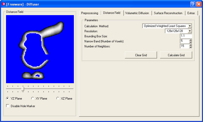
The distance field calculation initializes the octree data structure and constructs the signed distance function with the specified Resolution. There are several calculation methods implemented:
• Tangent Plane Estimation
• Optimized Weighted Least Squares
• Weighted Least Squares
• Next Point
Tangent Plane Estimation calculates the tangent plane of a given neighborhood in the least squares sense. The Optimized Weighted Least Squares calculation method makes use of the normal information to improve quality. This algorithm is a good choice when the input model is very noisy and no denoising filter is applied to the object. Weighted Least Squares should not be applied for large neighborhoods since it might generate artifacts; it is only used to compare with the optimized version. Next Point just calculates the distance to the next point resulting in a fast algorithm with poor quality. Normally the bounding box includes the object and the whole narrow band. In special cases it might be desirable to expand the Bounding Box Size (e.g. for offsetting). The Narrow Band is specified as number of voxels which define the computational domain. Number of Neighbors defines the neighborhood size for the calculation method. Calculate Grid is used to start the distance field calculation for the active object and with Clear Grid the volumetric grid is deleted. Note that this function is implicitly called when recalculating a grid. After the distance field computation is finished the slices of the volumetric grid can be seen on the left side. There are three buttons YZ-Plane, XY-Plane and XZ-Plane to switch between all three directions.
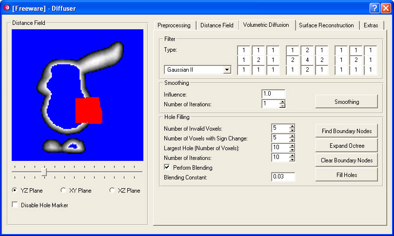
There are four predefined filters to choose from (3x3x3 box, 7-point plus, Gaussian I and Gaussian II). The filter values can also be edited to change the influence values. Only when applying an asymmetric filter differences can be noticed. Smoothing might be used to perform an isotropic volumetric diffusion over the whole narrow band. The influence of the operator can be adjusted from 0 with no influence to 1 with large influence. Note that smoothing can lead to a smaller resulting size because isotropic diffusion tends to shrink the object. To utilize the hole filling algorithm boundary nodes have to be identified. Per definition a boundary node is a node with at least one invalid neighboring voxel and one neighboring voxel with a sign change. Sometimes it is useful to increase these parameters to achieve better predictions. Boundary nodes are marked with red on the distance field display. The next step involves expanding of the octree. Because each hole is not treated independently the parameter Largest Hole has to be adjusted until all holes are covered with the red marker on the distance field image. To start the diffusion process Fill Holes has to be selected which depends on Number of Iterations. Clear Boundary Nodes should be used to reset the boundary node tags. Note that the red marker can be disabled by deselecting Disable Hole Marker on the left.

There are two possibilities to reconstruct a surfel collection from a given
distance field. The Elliptical Marching Cubes algorithm produces a
dense and accurate sampling of the distance field. Further, it is possible to
extract the iso-surface at a user-specified level when changing the Offsetting
value. Note that the extraction is limited to the narrow band, thus when extracting
the surface with a too high or too low offsetting value holes might appear.
For the particle simulation the user has to specify the Target Size
and adjust Variation Influence. Then the Initialize Particle Simulation
button should be clicked. The algorithm uses a kd-tree and is dependent on Number
of Neighbors, Iterations, a constant Force Scale and
a Damping value. Note that the quality of the resulting particle simulation
also depends on the narrow band size. The moving least squares projection procedure
can be used to improve quality of the particle simulation. The value Number
of Neighbors defines the neighborhood size for all computations. Recalculate
Normals computes the normals of the neighborhood in the weighted least
squares sense. When deselecting this option the current normal is used to find
the local reference domain. When Approximation is enabled it is assumed
that the local reference plane passes through the point. This reduces computation
time but generally results in a loss of quality. The points are projected either
on a 3rd Degree Polynomial or 4th Degree Polynomial. Adjust
Normals should be selected to use the normal of the polynomial approximation
rather than the original normal. Finally, the procedure is started when confirming
with Projection. Note that the non-linear equation system introduces
computational complexity (i.e. when Approximation is disabled).
To guarantee coverage of the surfels the Sampling plug-in should be
applied. Good results can be achieved using the k-nearest neighbors or the approximate
Voronoi cells methods.
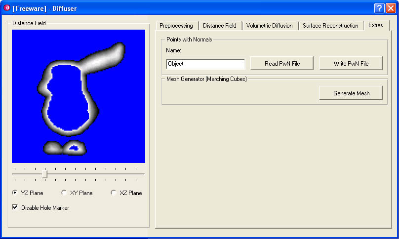
The module Extras contains two additional features. Points with Normals is an ASCII file format which stores the number of surfels, their spatial information and their normals. Note that all other information is dismissed. Additionally, there is an option to extract a mesh-based representation of the distance field using the marching cubes algorithm. The supported file format is RAW, which stores the coordinates of the triangles in an ASCII representation.