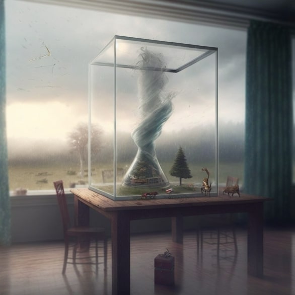
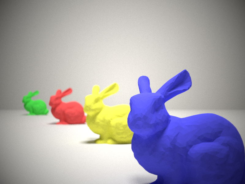
Motivational Image
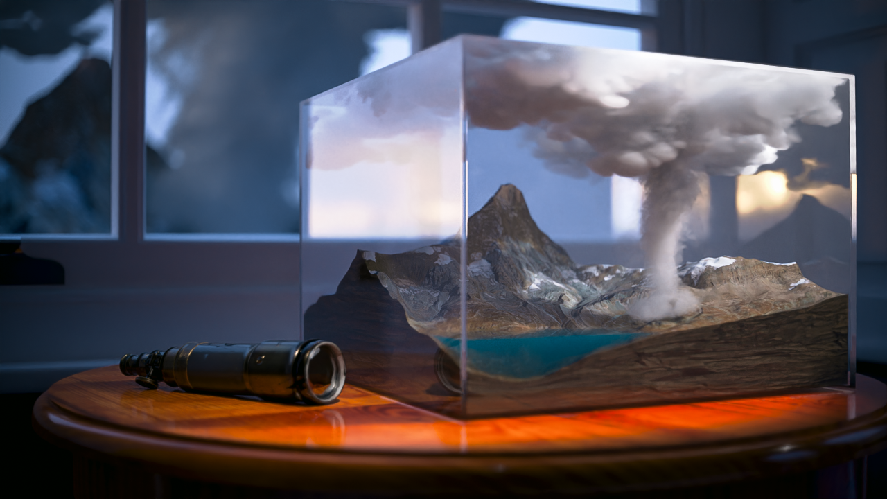
Our proposal was to render an image of a tornado inside a glass box on a table. The tornado would be modelled with heterogeneous media. We would model the materials of other objects on the table and inside the box with the Disney BRDF. The scene would be lit with an environment map and a spotlight emitter.
Now we make a biref description and explanation of the implemented features for each of the members. Each of us has implemented exactly the 60 points as in the sent proposal. The XML files used for validation scenes can be found in folder validation/ of our code submission ready to be rendered with our Nori implementation. Our project scene project.xml can be found in the folder project/, and it is also ready to be rendered with our implementation.
Dario Mylonopoulos
Environment map emitter (15 pts)
Updated files
-
envlight.cpp -
dpdf.h
Description
The environment map is implemented following the approach described in chapter 12.6 and 14.2.4 of the PBRT book.
A new emitter type EnvironmentEmitter was implemented in the file envlight.cpp, a new utility class for sampling from 2D discrete distributions was implemented in dpdf.h and a new method for continuously sampling from a Distribution1D object was added in the same file.
The Distribution2D is used for imporatnce sampling the environment map emitter based on the luminance of each pixel weighted by the sine of the spherical angle \(\theta\) to take into account for the distortion of the equirectangular projection.
This new emitter type is threated differently from other area emitters in the integrators since it is hit whenever the ray does not intersect any geometry. Therefore when parsing the scene this type of emitter is saved in a member variable of the scene which can be queried with a new getEnvironment() method.
This emitter is also included in the list of emitters so that it can be sampled normally when performing Next Event Estimation.
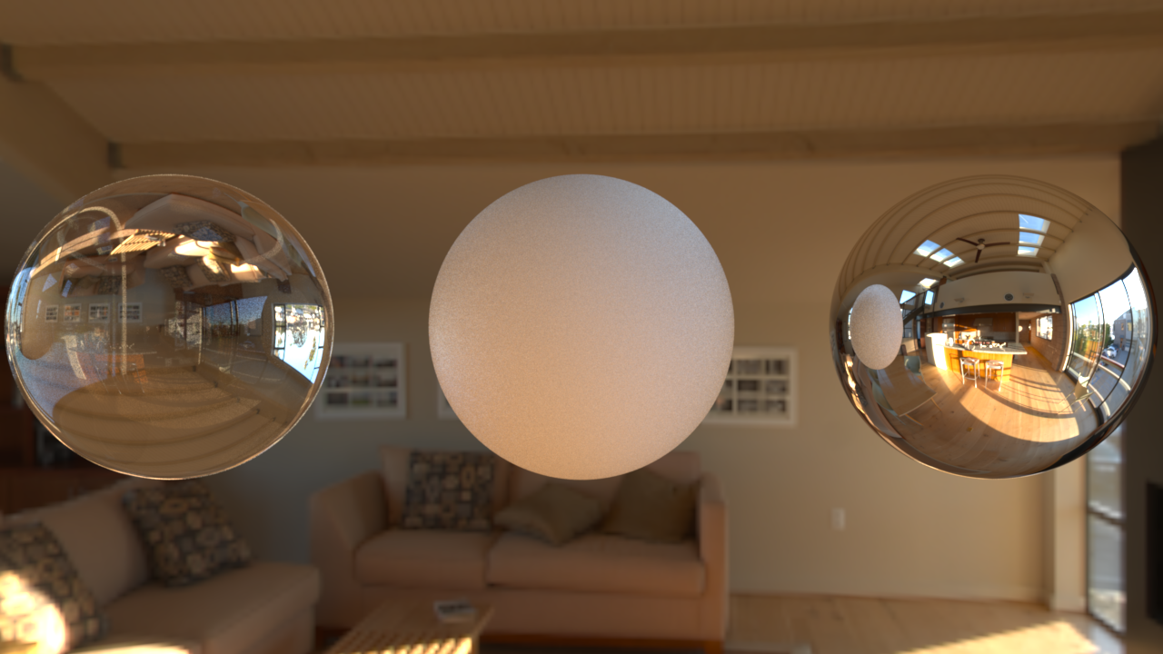
Validation
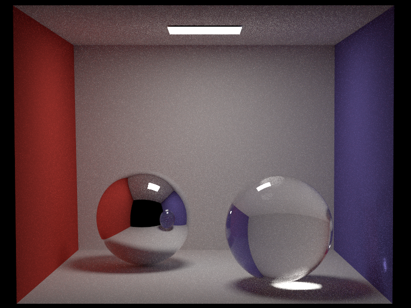
We compare our implementation with Mitsuba 3 on a test scene with spheres lit by the environment. The materials are (from left to right) dielectric, diffuse with a white albedo and a perfect mirror.

Disney BRDF (15 pts)
Updated files
-
disney.cpp -
warp.h -
warp.cpp
Description
The disney BRDF is based on the paper "Physically Based Shading at Disney - Burley 2012". The BRDF is implemented in disney.cpp and methods for sampling and computing the PDFs of the GTR1 and GTR2 distributions have been added to warp.h.
The following parameters have been implemented: roughness, metallic, specular, specular tint, clearcoat and clearcoat gloss. Therefore the diffuse, main specular and clearcoat lobes were implemented.
Importance sampling of the BRDF is implemented by first choosing to sample the diffuse, specular or clearcoat lobe
with the following weights (which are normalized for sampling):
$$
\begin{align}
&w_\text{diffuse} = 1 - \text{metallic} \\
&w_\text{specular} = 1 \\
&w_\text{clearcoat} = 0.25 \cdot \text{clearcoat}\\
\end{align}
$$
and then sampling a cosine weighted hemisphere for the diffuse lobe, and proportionally to the microfacet normal distribution term D for the clearcoat and specular lobe, using the GTR1 and GTR2 distributions respectively.
Validation
We compare our implementation with Mitsuba 3. We have 6 rows of spheres, each one has the tested parameter varying from 0 to 1 with the others held constant. From top to bottom the parameters are roughness, metallic, specular, specular tint, clearcoat and clearcoat gloss. The scene is lit by the environment map and by a point light.
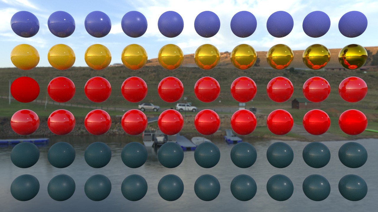

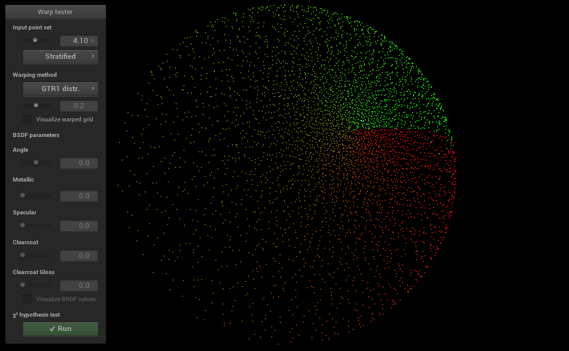
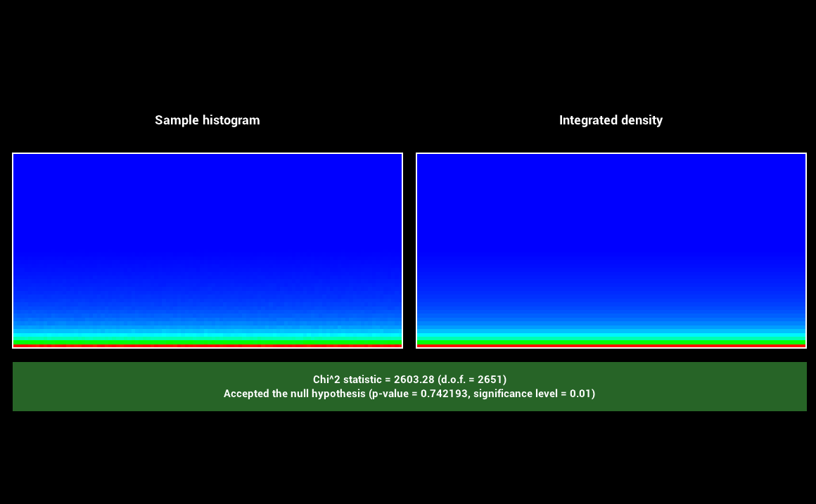
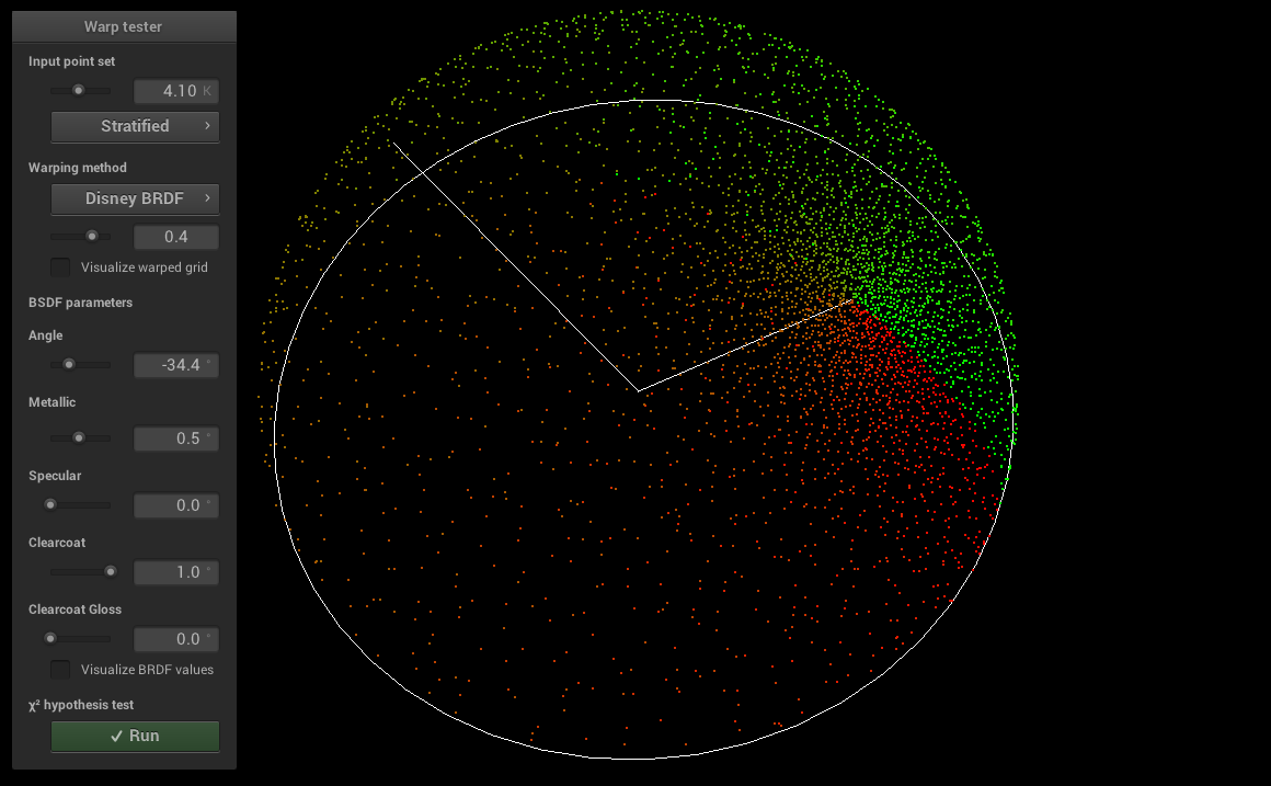
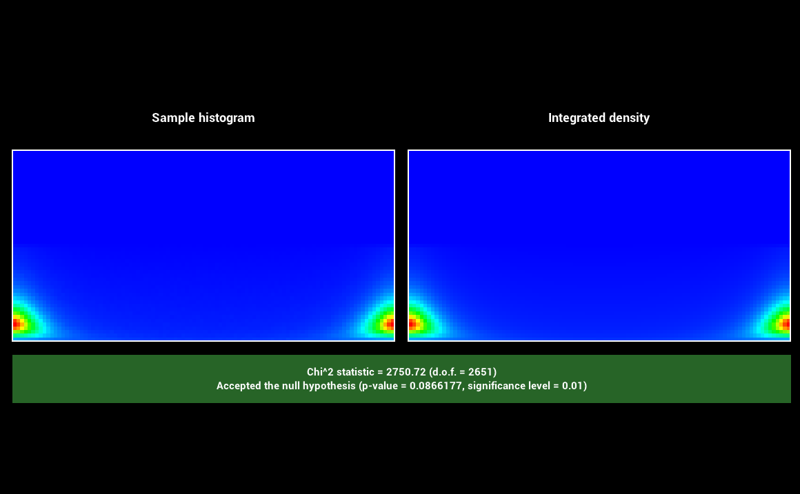
The specular and clearcoat lobe use the GTR1 and GTR2 distributions in their D term. Those and the BRDF itself have been tested with the warptest program to ensure that sampling procedures matched the corresponding PDFs. We include screenshots from warptest
for the two distributions and for the BRDF.
GTR1:
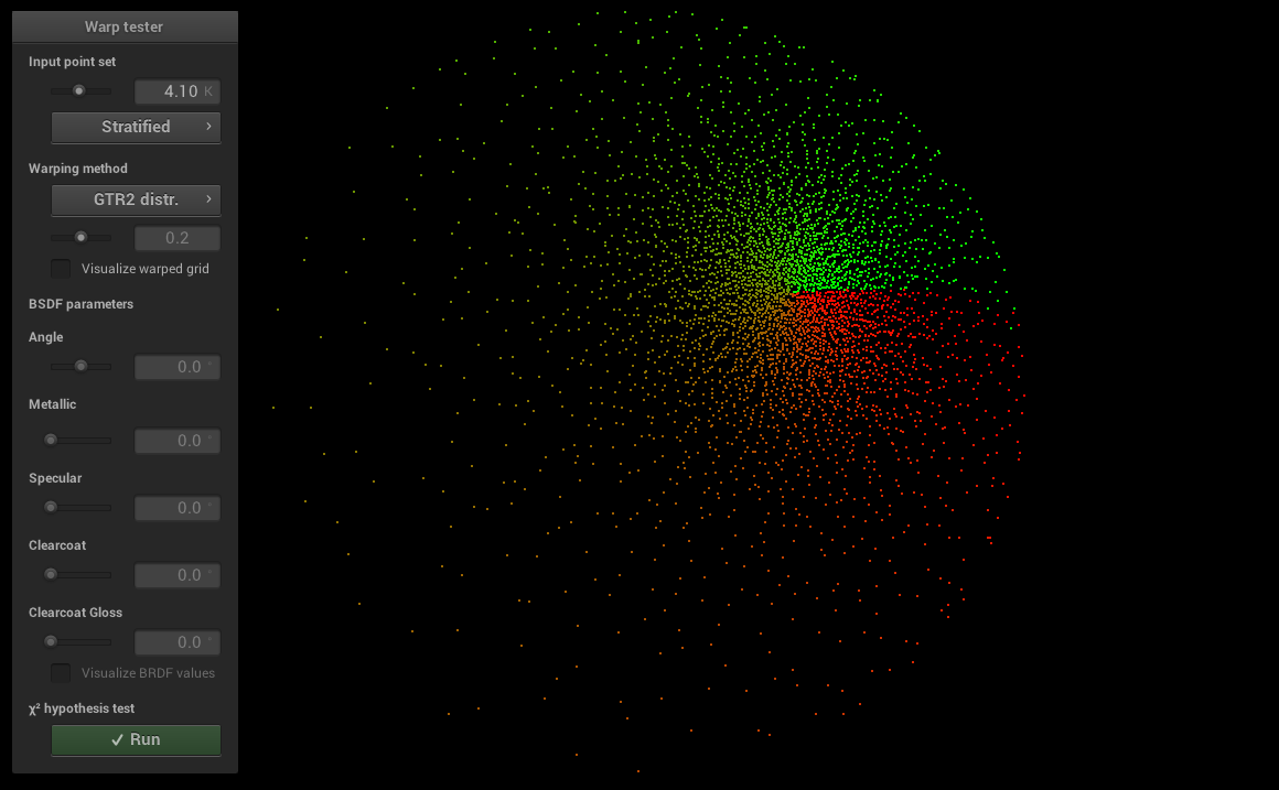
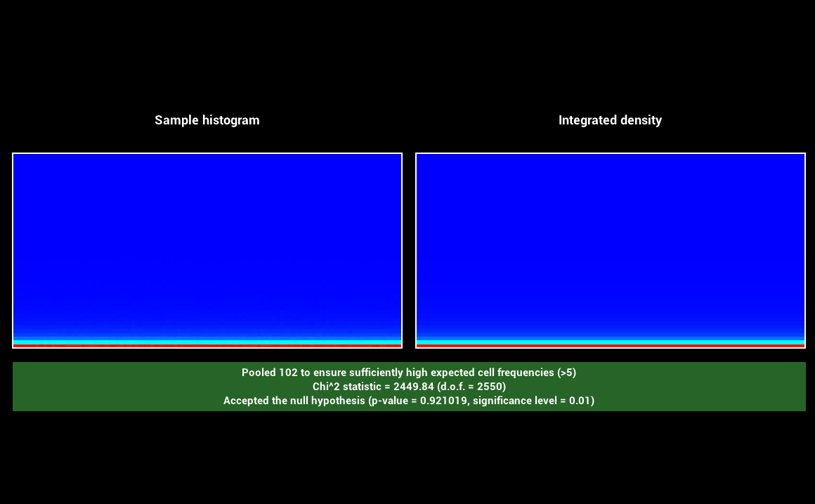
GTR2:
Disney:
Images as textures (5 pts)
Updated files
-
image_texture.cpp -
disney.cpp
Description
TheImageTexture type is implemented in image_texture.cpp. A templated class to load and sample from a texture has been implented with 3 specializations: one for loading colors (converting from sRGB to linear) and two for floating point values (1 channel and 3 channels, without sRGB conversion)
that are useful for roughness/metallic texture maps and normal maps which are usually not stored in sRGB space. The disney BRDF was updated to supports loading albedo, metallic and roughness values from textures.
Validation
We compare with Mitsuba the rendering of a model using the disney BRDF with albedo, metallic and roughness texture maps.

Normal mapping (5 pts)
Updated files:
-
shape.cpp -
mesh.cpp
Description
Normal maps have been implemented inside the Shape class inshape.cpp. A convenience method was also added to the Intersection class to modify the shading frame with the normal map associated to the intersected mesh.
Additionally support for computing a continuous tangent based on the UV coordinates of a mesh frame was added to the Mesh class in mesh.cpp in the Mesh::setHitInformation method.
A normal map can be associated with a mesh by adding a texture named "normal" to the mesh object. The normal map is then sampled and used to update the shading frame after an intersection with a mesh is found by calling the method Intersection::applyNormalMap().
Validation
We compare with Mitsuba the rendering of the same model used previously for testing texture maps, comparing with and without normal mapping. We can see how normal mapping can add a lot of details in areas that were previously flat.

Mip maps (10 pts)
Updated files:
-
image_texture.cpp -
ray.h -
perspective.cpp -
shape.cpp
We expanded the
ImageTexture in image_texture.cpp to compute the mip pyramid when a texture is loaded and perform trilinear interpolation when sampled. To choose which mip level to sample we need to keep track of ray differentials.
We follow approach described in chapter 2.5.1 of the PBRT book and introduce a subclass of Ray3f called RayDiff3f in ray.h that keeps track of ray differentials.
We generate rays with differentials in the sampleRay() method in perspective.cpp and when an intersection is found we compute UV coordinates differentials in Intersection::computeDifferentials() in shape.cpp which are then used to compute
the desired width of a texel and choose the corresponding mip level.
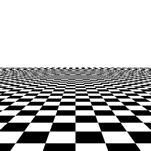
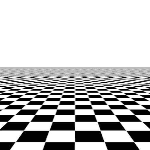
Validation
We validate our implementation by rendering a checkerboard pattern with and without mipmapping. We also show a debug visualization of which mip level was sampled at each pixel.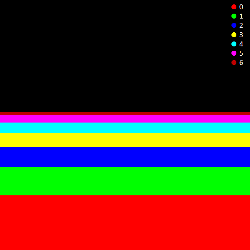
Open Image Denoise (5 pts)
Updated files:
-
oidn.h -
block.h -
block.cpp -
render.cpp
We integrated the Open Image Denoise library into the renderer for denoising. The implementation is in the file
oidn.h, which calls the library for denoising the bitmap passed in. Open Image Denoise also supports denoising with albedo and normals feature buffers to improve the denoised image.
To keep track of this information we added two arrays in the ImageBlock class called albedo and normals respectively that keep track of these additional channels in block.h and block.cpp. We also added two parameters for returning the albedo
and normal at the first hit to the Integrator interface and to all integrator implementations. To get the albedo at an intersection we also added a albedo() method to the BSDF interface and respective implementations.
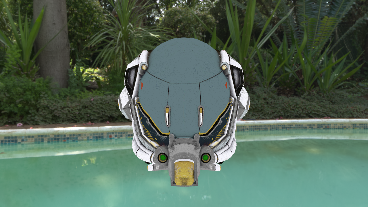
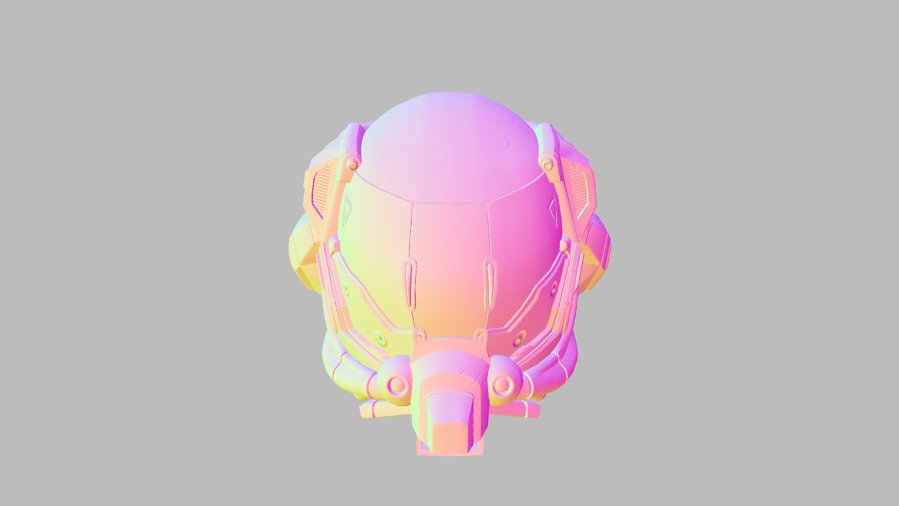
Validation
We validate our implementation by showing the results before and after denoising on an image rendered with 8 samples per pixel. We also show the feature buffers containing albedo and normals (remapped from 0 to 1).

Euler cluster (5 pts)
Updated files:
-
main.cpp -
euler/compile.sh -
euler/run.sh
-c as a command line flag to Nori. If the flag is given a RenderThread is created directly without a NanoGui window. The implementation is in the Nori main.cpp file.
We also created two bash scripts in the euler directory that can be used to compile and run nori with the batch system of the cluster.
Validation
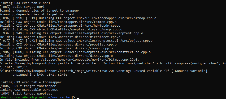
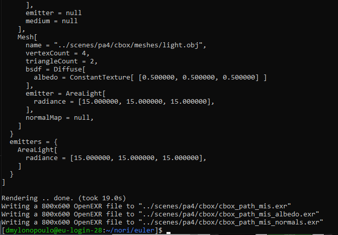
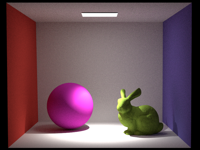
We validate our implementation comparing the same scene rendered locally and on the euler cluster. We also show screenshots of the output of the compilation and rendering jobs on the cluster.
Sergio Sancho
Spotlight (5 pts)
Relevant files:
src/spotlight.cpp
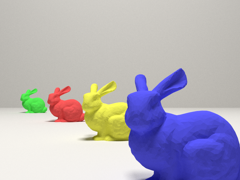
(The Stanford bunny model has been used for validation).
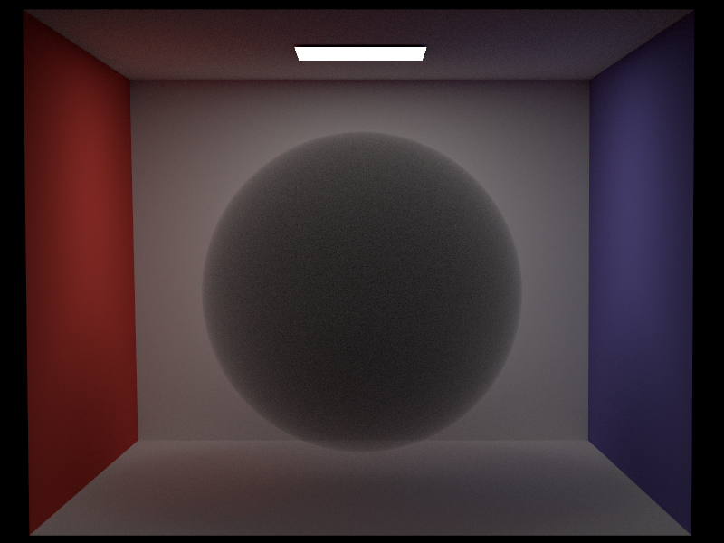
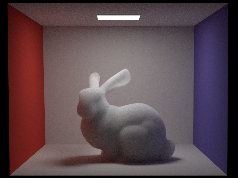
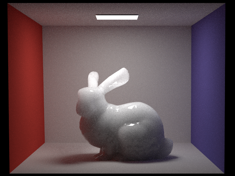
In our project we would like to illuminate a specific region of the scene in order to remark the importance of some objects in it and to be able to control the region of lighting. A spotlight is a good choice to achieve that. It extends the normal pointlight by introducing a falloff which allows to perform illumination on a cone, with its vertex at the light origin position.
The implementation is very straightforward: from the scene file, we need to specify a maximum angle of illumination and a smaller angle where the falloff starts. We also need a target position that we want to light and that will give us the direction of illumination of our light. In our spotlight class, we will compute as usual the vector \(\omega_{i}\) as we do in the point light, but then we will compute the dot product with the spotlight direction to be able to compare the angles in form of cosines. We will multiply the intensity of the light by 0 if the evaluated object leaves outside the cone (completely dark), by 1 if it is inside and it is before the staring of the falloff, or by a specific falloff coefficient if it is the middle. Function getFalloff() handles these cases.
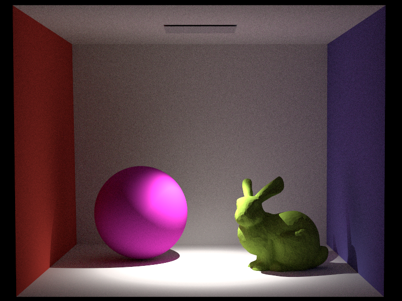
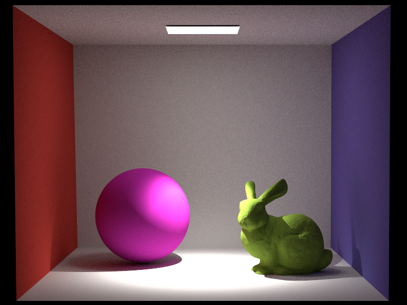
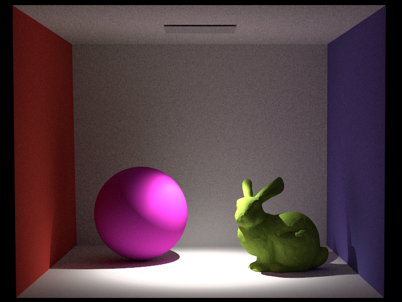
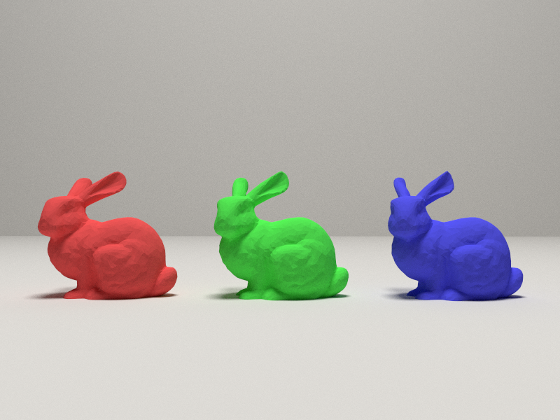
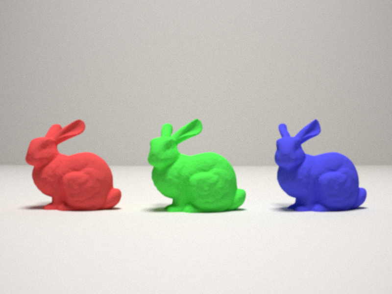
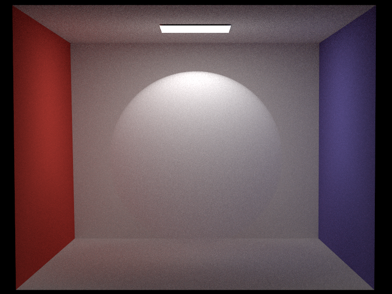
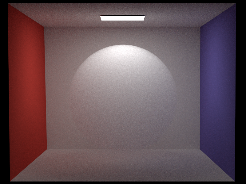
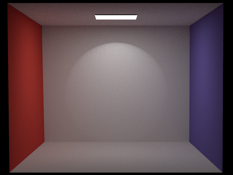
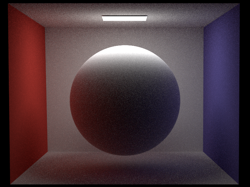
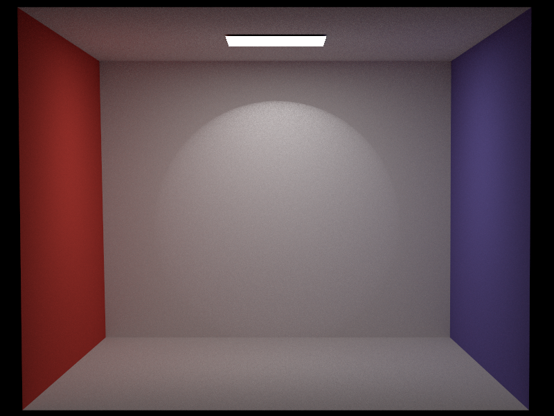
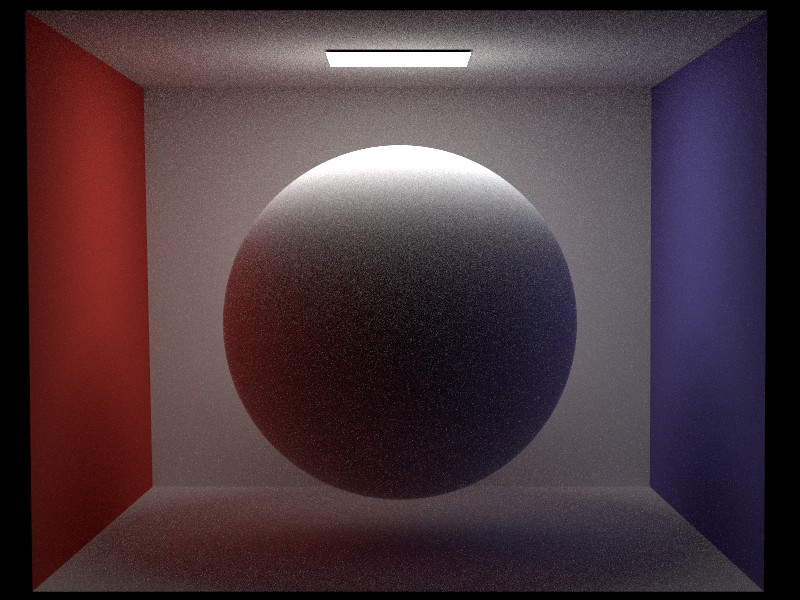
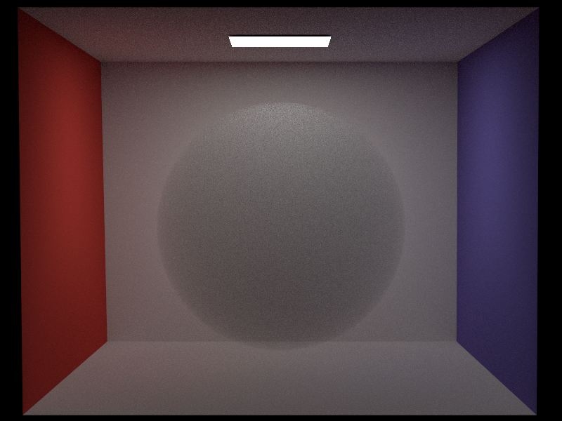
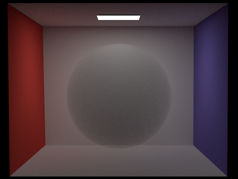
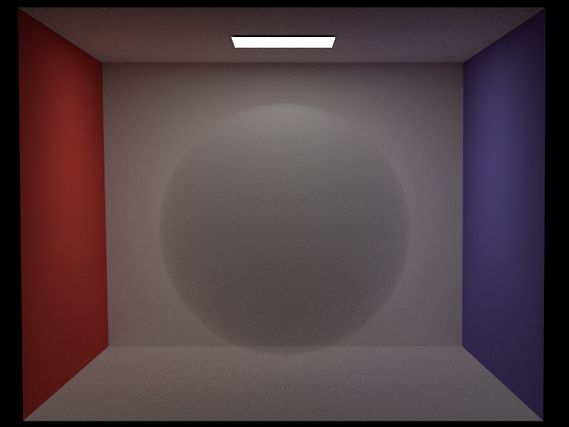
Now we show some results and comparisons of the spotlight. We compare the spotlight in a scene with an extra area light and without (only with the spotlight). Our implementation is compared against PBRT v3.
Realistic camera (15 pts)
Relevant files:
src/realistic.cpplenses/*.dat
The basic camera that nori implements follows a pinhole camera approach where the rays go through a single point in their way to the film plane, limiting some interesting effects, such as depth of field, that happen in real cameras where this ideal situation is not physically plausible. One approach is to model this following the thin lens model, where an additional ray projection into an aperture plane takes place, allowing to control the depth of field based on the amplitude of the aperture and the distance of this plane to the film.
However, we have decided to simulate a realistic camera following the same procedure as PBRT book in Section 6.4 and the paper by Kolb et al. ("A realistic camera model for computer graphics.", 1995) in order to achieve the real effects that one could obtain in real photography. In this model, we use a lens system formed by a group of individual lens elements that are aligned with the optical axis. As in other camera models, we will generate rays sampling at some positions on the film plane. The difference is that in this case we will let our rays to propagate through the lenses, one by one, and change their direction in terms of the refraction that takes place at each element. Rays might also terminate before leaving the camera if they hit an opaque part of a lens element. Simulating the camera rays paths in this way using a well-designed system of lens elements will not only recover the image seen from the camera view, but also introduce effects like depth of field, bokeh effect, distortion, vignetting, etc.
The following image shows a representation of one of these lens systems.

Each of the lens elements is defined by a curvature radius, a thickness, a refraction coefficient, and an aperture radius. The aperture stop is also part of these elements, and we can control it through a parameter to get more or less light into the sensor. We import the data for a specific lens system stored in a file and construct the camera. We have taken the lens files from the PBRT v3 implementation. Since the user decides the focus distance through a parameter, the constructor figures out the position of the lens system with respect to the film position on the optical axis using the method focusThickLens() and computing the cardinal points.
We could then use our sampling rays function to sample rays on the film and let them simulate the path with the method traceLensesFromFilm(). However, as the book explains, we would be wasting many ray samples that would not end up exiting the lens system. Instead, we also sample the exit pupil. The exit pupil is the region on the rear element of the lens system where the rays that can exit pass. This region changes depending on the position of the film plane in a symmetric way, so we can compute the area for this region in the constructor. When we generate the rays, we will sample the film and the corresponding exit pupil region. It is also important to mention that in this camera model we have a physical film with an actual size, parameterized by its diagonal.
Below we compare the effect of using the realistic camera model in our implementation. We use the normal perspective camera using the pinhole model and the realistic camera for the same scene: the 3 effects of interest as indicated in the project proposal (depth of field, lens distortion and vignetting) are clearly visible within this unique example. For the realistic camera, we have used the D-GAUSS F/2 lens file working with a film of 50 mm of diagonal size.

In the previous example we see that our implementation achieves the desired effects when compared with the normal camera. Now we will validate our implementation with the PBRT v3 implementation.
Now we show another example scene using the fisheye lens file (Muller 16mm/f4 155.9FOV fisheye lens) for a film of 10mm of diagonal size. We compare our implementation of the realistic camera with the normal pinhole camera to show the effect of distortion in the result.
Heterogeneous Volumetric Participating Media with Path Tracing (30 pts)
Relevant files:
include/nori/grid.hinclude/nori/medium.hsrc/trivial_bsdf.cppsrc/phase_isotropic.cppsrc/homogeneous.cppsrc/homogeneous_ms.cppsrc/heterogeneous.cppsrc/heterogeneous_ms.cppsrc/path_mats.cppsrc/path_mis.cppsrc/scene.cpp
(The Stanford bunny cloud VDB has been used for validation).
We have implemented participating media following the "Production volume rendering" Siggraph Course (Fong et al., 2017). We liked this approach instead of the one followed by PBRT because it organizes the integrator in a slightly different way. Instead of dealing with media scattering in a specific way using a new Phase class to sample from, it implements the phase functions as a BSDFs. With that, the same path integrator can be used with some minor modifications. For instance, we do not have a geometric term (cosine of theta) when adding the radiance contribution from a direction. But overall, we integrate in the medium in a similar way as we integrate in surfaces: we sample a distance to a next intersection (in the case of participating media, it will be a scattering "virtual" intersection chosen by our technique of distance sampling) and on that point we do next event estimation (direct lighting to a random emitter) and we sample a direction with the BSDF (in participating media, the BSDF will implement a phase function). We use multiple importance sampling to add these contributions, and then continue the recursive integration, that is, we sample a new distance following the sampled direction as usual.
The file medium.h provides the class interface for the medium. We store the medium on a Shape object, meaning that the specfic shape contains a medium inside. We have implemented a trivial BSDF to add to a mesh in order to denote an invisible surface. The ray tracks the medium in which it remains, and a procedure in the path integrator checks that after a intersection the medium of the ray changes accordingly. The path integrator (for instance path_mis) will, for each iteration, either ask for the next intersection in the scene if it is not travelling thruogh a medium, or use the integrate(..) method of the corresponding medium if it is travelling through it. Both methods will return the next intersection point where scattering should occur, either at a surface intersection or at a "virtual" scattering intersection on the medium. The next event estimation algorithm to compute direct lighting has also been extended to account for transmittance along the ray using the method computeTransmittanceRay(..) in the Scene class.
Below we show the general equation without emission to do volume rendering, where we can appreaciate how similar it is to the normal rendering equation.
\begin{equation} L(\vec{x}, \vec{\omega})=\int_{t=0}^{d} T(t)\left [ \sigma_{s}(\vec{x}) \int_{S^2} f_p (\vec{x_t}, \vec{\omega}, \vec{\omega}') L (\vec{x_t}, \vec{\omega}') d\vec{\omega}' \right ] dt + T(d) L_d(\vec{x_d}, \vec{\omega}) \end{equation}Note that in our implementation the user parameters for a volume are the scattering albedo and the extinction coefficient, whereas in PBRT they use the absoption and scattering coefficients. One can easily convert between these parameters. We have also implemented the version of single scattering, where a single scattering event is sampled in the medium and next event estimation is performed there. In this version, volume integration takes places only inside the medium object, and the path integrator does not deal with scattering events. In multiple scattering, as mentioned before, the path integrator also integrates the different path segments inside a volume.
Homogeneous volume
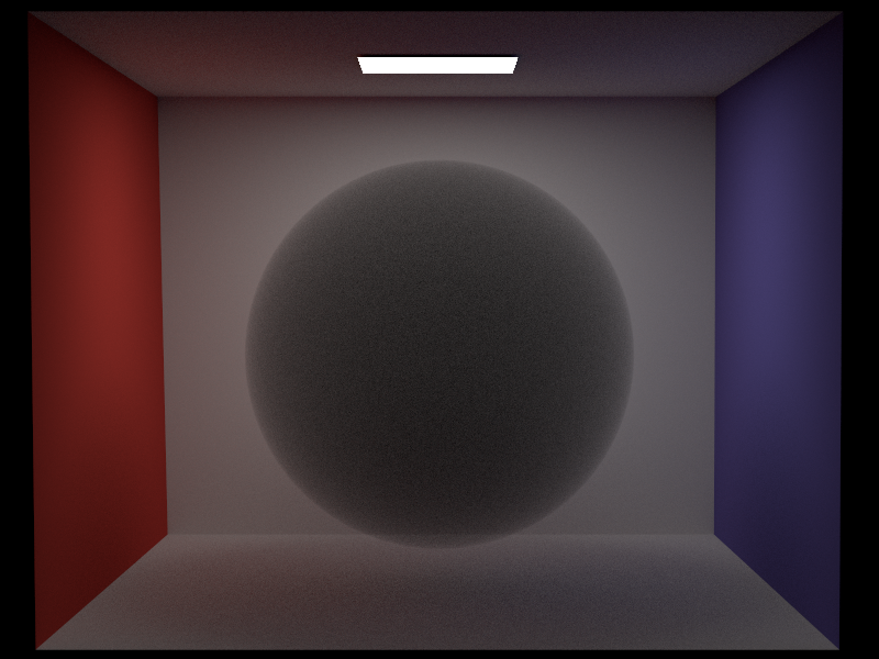
Now we will compare our multiple scattering homogeneous volume implementation with Mitsuba for the absorption only sceneario (that is, an albedo of 0) and for scattering only (albedo of 1) with an extinction coefficient of 2 and 256 spp.
In the follow example we set the scattering albedo to 0.95 and we show how it aeffects to change the extinction coefficient from a low (0.5) to a high one (20) with 256 spp.
We compare now our implementation of multiple scattering homogeneous volume (128 spp) with our implementation of single scattering and with the Mitsuba reference for an albedo of 0.25 (some absorption and some scattering).
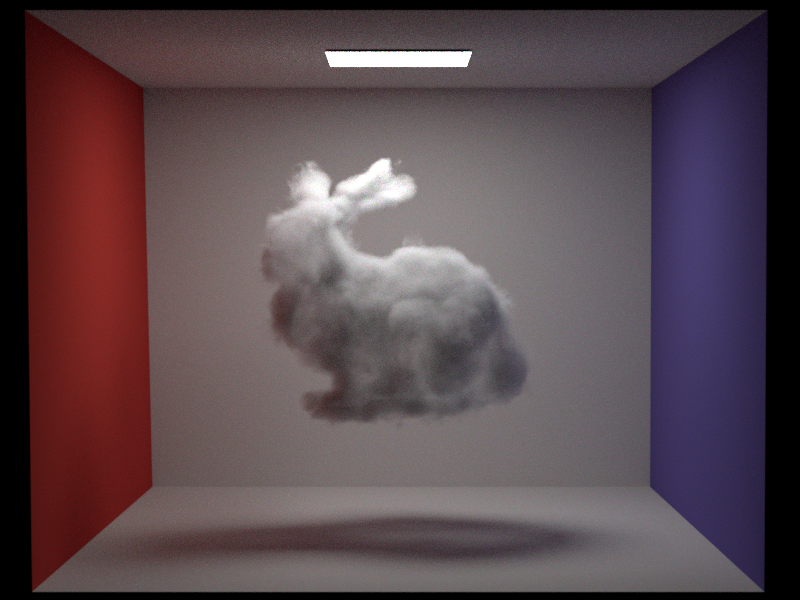
Now we show a comparison of a homogeneous volume in the shape of a bunny mesh for multiple scattering.

Our implementation also allows to set a BSDF as the interface of the medium. Below we compare the result of using a trivial BSDF which does not interact with the ray, and a dielectric interface.
Heterogeneous volume
(Note: We use Nvidia NanoVDB in our implementation and to transform from OpenVDB to this format).
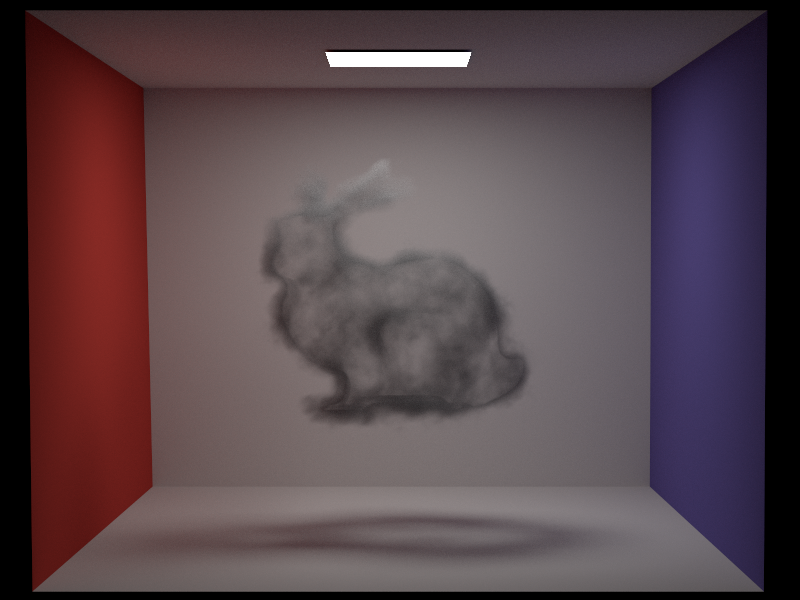
We can see now our implementation of the heterogeneous participating media in nori compared with the implementation of PBRT v4. In both cases we use a NanoVDB file of the bunny cloud. However, and since the our implementation does not follow the PBRT implementation, volume grid transformation is hadled in a different way. This is the reason why the scale and position between both images does not fully correspond (since we had to place it manually). Nevertheless, the actual result is almost identical.
(Note: We used PBRT v4 for convinince here, since it can work with NanoVDB, which is the same format that we use in our implementation, and therefore we can use the same volume file. However, new version of PBRT changes the volume integrator to the null-scattering path integral formulation of Miller et al. ("A null-scattering path integral formulation of light transport", 2019), while we use the delta tracking approaches in the comparison, and this is the reason why PBRT v4 looks more converged).

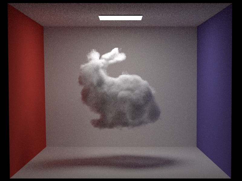
Now we compare our implementation of the multiple scattering heterogeneous volume with a high extinction coefficient and high scattering with a lower extiction coefficient and higher absorption.
Delta tracking, ratio tracking and ray marching (10 pts)
Relevant files:
src/heterogeneous_ms.cppsrc/heterogeneous_ratio_ms.cppsrc/heterogeneous_raymarching_ms.cpp
Note that in both cases we do not introduce bias, and they should converge to the same result. Another methods that we have implemented, both for distance sampling and transmittance estimation, is ray marching, following the explanation on the slides. In this case the process is completely different, since the transmittance is estimated dividing the path of a ray inside a volume in small segments of a specific step size. Then we treat each of this segments as a homogeneous small volume with a fixed extinction coefficient. We perform distance sampling in a similar way, advancing small steps until a random transmittance is achieved, and at that point we do scattering. However, this method introduces bias, but it has the advantage that we can control the step size and therefore the computation time.
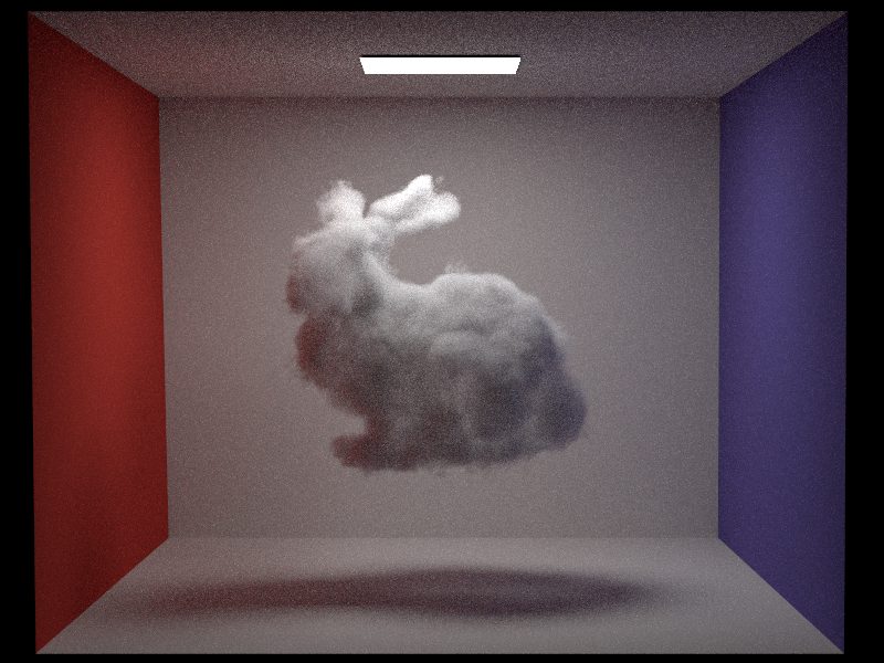
We show a comparison below of the bunny heterogeneous media for 64 spp. As expected, delta tracking is faster and it took 6.5 minutes, while ratio tracking took 7.6 minutes on the same machine. The difference is very subtle, but is noticeable in the noise of the roof and the volume. Ratio tracking achieves a better convergence for the same number of samples and we see that fireflies on those areas are less bright than with delta tracking. We provide a zoom in of a region of the volume to better appreciate the difference. We also show the comparison with ray marching distance sampling and transmittance estimate using a step size of 0.01.


Other implemented features (not graded)
We have additionally implemented some features to use in our final image. We have implemented the Henyey-Greenstein anisotropic Phase Function to achieve a better effect on the clouds. The implementation can be found in src/phase_hg.cpp.
Project Image
Resources for project scene:
- Room scene with models
- Telescope model
- BlenderGIS plugin (3D terrain from geographic data)
- JangaFX VDB files to create the tornado
- Quixel Megascan rock texture.
We have used the previously described methods to compose our final image for the project. A room is shown where a small environment formed by a terrain with a lake and a tornado is contained inside a glass box, showcasing the theme of out of place. The terrain shows a mountain that has been modelled using the real cartographics data of the Matterhorn. Outside the window we can see the same mountain and also the tornado as inside the glass, playing with the concept of recursion. We thought it was interesting to show recursion in a scene that it is rendered using the recursive Monte Carlo path tracing method. A telescope completes the image.
The tornado has been modelled using the implemented heterogeneous media that takes NanoVDB files. We have used the JangaFX free VDB assets and Houdini Apprentice version to combine all of them to form the tornado cloudy shape. Below we show an image of how we have deal with that in Houdini.
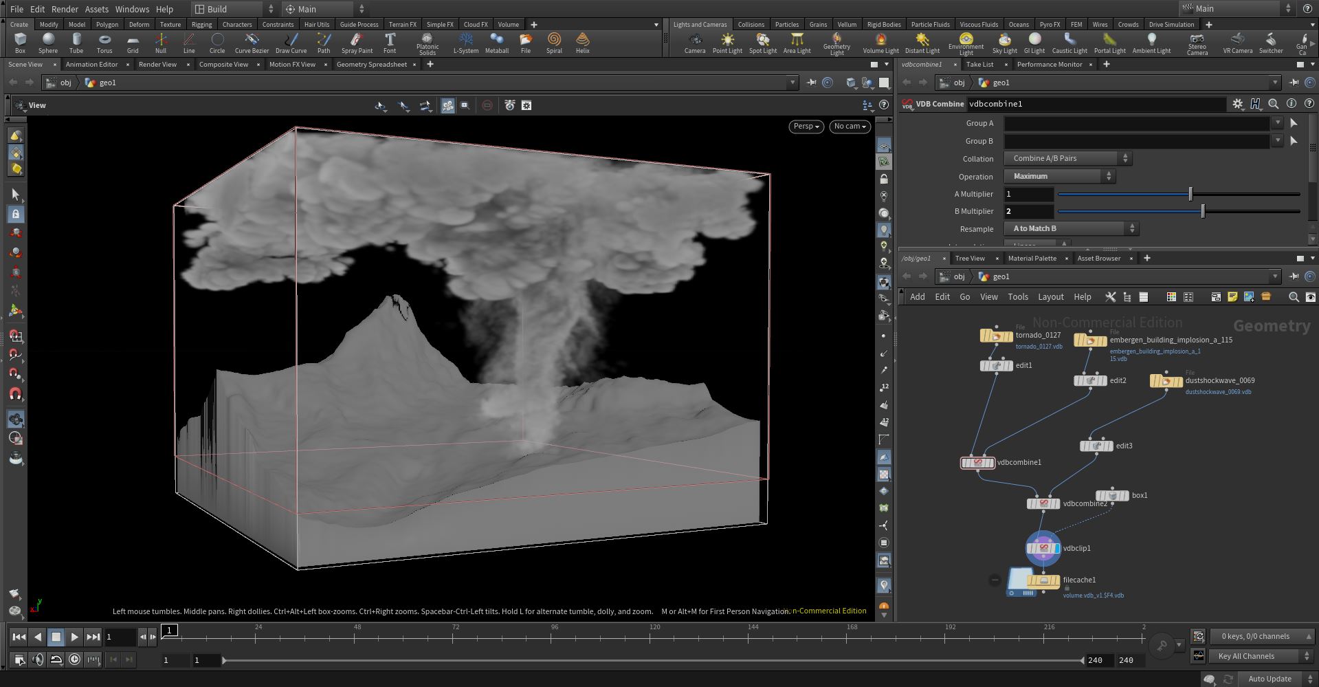
As mentioned before, we have used the delta tracking approach for the tornado inside the box, and the ray marching with a larger step size in the tornado outside, since in this one we are not interested in the precision of the result but on achieving a less expensive computation. In terms of participating media, we have also used an homogeneous media with a dielectric BSDF to simulate the effet of water in the lake, giving a bluish color with the RGB scattering albedo.
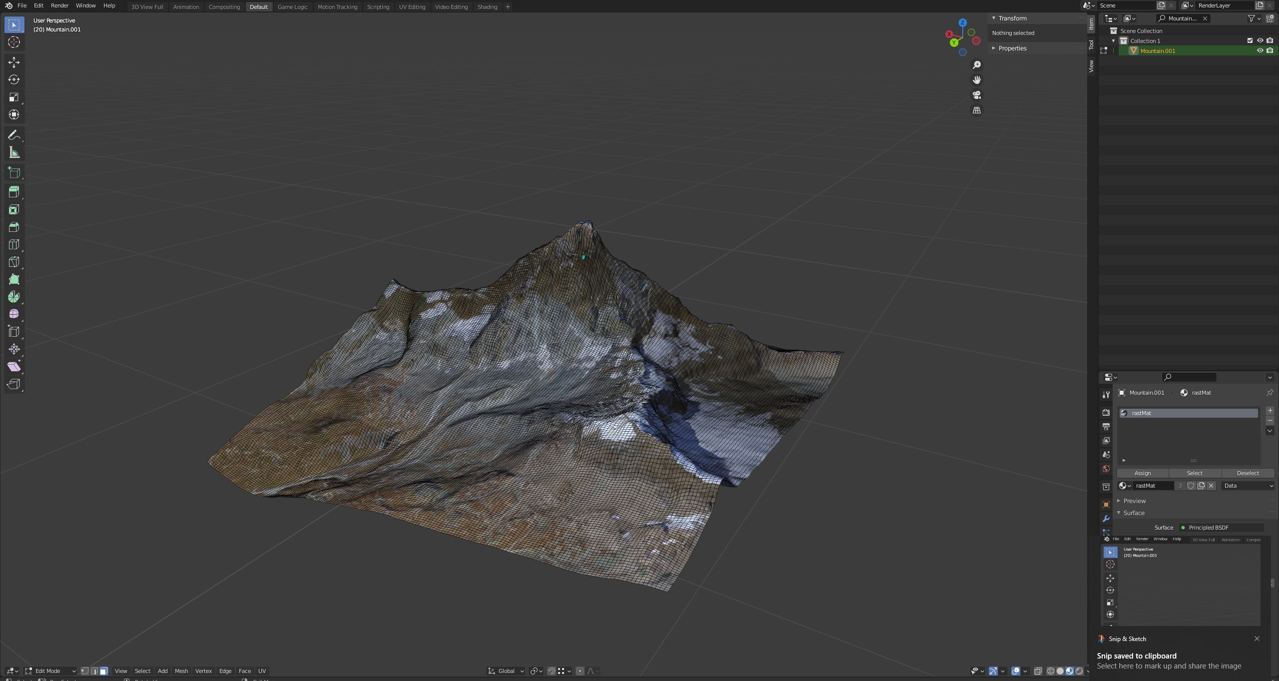
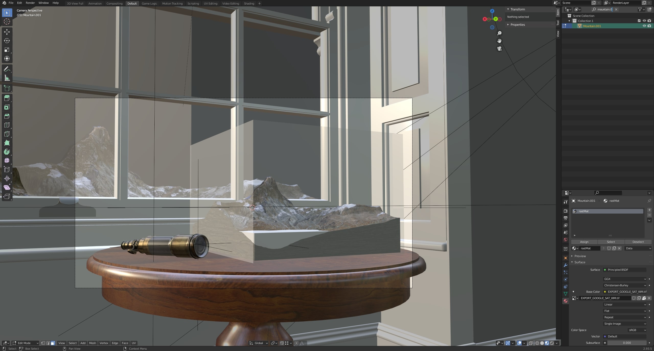
We used the plugin BlenderGIS to create a model of the Matterhorn mountain. The plugin allows you to use satellite images as textures and real world elevation data to create a heightmap which is then used to displace the mesh. We then cut out a square of this terrain and modelled and textured the sides of the patch. Below we show a screenshot of the geometry and texture of the mountain.
We also used blender to place the camera and the elements in the scene and export .obj files for rendering in Nori.
Final Image