Subsurface Scattering with Photon Beam Diffusion
Effect of the Feature
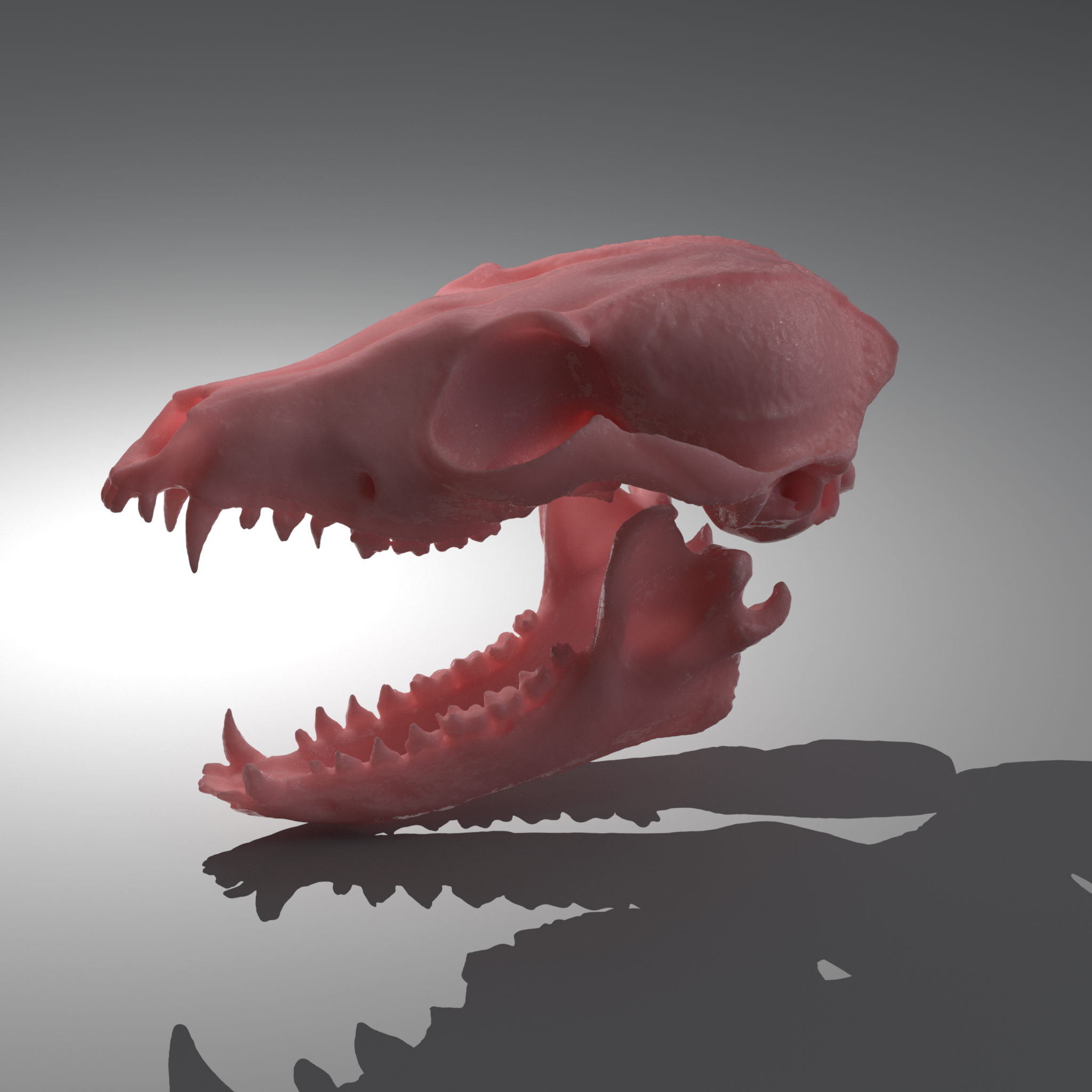
The effect of subsurface scattering (SSS) describes the bouncing of light inside a medium before leaving it again. This leads to a "soft" looking material, like wax, milk or skin. While it is in theory possible to simulate this phenomenon by actual Monte Carlo path tracing (i.e. each scattering event is simulated), this approach is not feasible as it leads to very long render times. Instead we perform a so-called diffusion approximation.
Technical Implementation
Overview
For this project, we implement the approach of photon beam diffusion (PBD) by Habel et. al.
For large parts, we follow the PBRT-v3 implementation which implements the same approach. We also report on how we deviate from PBRT in this report.
The core of the implementation is a lookup table to store the intensity of the SSS as a function of the SSS-parameters and the radius from the incident/outgoing point.
The table and the bulk of the implementation can be found in src/bssrdf.cpp and include/nori/bssrdf.h.
As we cannot accurately reproduce the material setup of PBRT due to complex layering and Mitsuba does not provide an implementation of PBD, we try to qualitatively compare the effects of subsurface scattering using the closest equivalent material in Nori (dielectric).
Parametrization
To avoid tedious parametrization over different scattering coefficents, we adapt the approach to define the mean free path and perform a inverse CDF lookup to find the corresponding SSS-parameters sigma_s and sigma_a. This implementation can be found in subsurfaceFromDiffuse() in bssrdf.cpp
Changes to the Path Tracing Process
For path tracing with subsurface scattering, we have to heavily adjust the path tracing approach in order to prevent code duplication, as we are now performing multiple importance sampling in two different locations (at the entering intersection and the leaving intersection). We therefore extract the BSDF- and emitter sampling into a separate function directMis. To check, whether we the last bounce was a transmission into the material, we add the property isTransmission to the BSDFQueryRecord. In transmissive BSDFs like Dielectric, we set this property to true in case of a refraction.
Sampling Incoming Positions and Computing Intersections
One place where we deviate from the PBRT implementation is the sampling of additional intersections. While PBRT does dynamically add new intersections to a list, we define a maximum for the number of intersections and only check that many times. In the current version, this maximum is set to 6. The core of the the photon beam diffusion is the sampling of a new point which corresponds to the location where a ray enters the object before leaving at the sample origin. A very nice visualization of the process of sampling the incoming point close to the outgoing point can be found in the PBRT Book, Figure 15.11. After sampling the incoming point (pi), we need to calculate the contribution of the subsurface scattering positional component. The nice thing about this approach is, that the sampling of the positional component can be performed independently and then multiplied. The influence of the sampled point pi is purely defined by the distance between the outgoing intersection (its) and the incoming intersection (pi). This evaluation is performed right after pi is sampled using the eval_sp(pi,po) function which performs a lookup in the table already described.
Sampling the Directional Component
As said already is the directional and the positional SSS-component multiplicatively connected. To sample the directional component, we add an additional BSDF (DirectionalSubsurface) that is added to each object to the dirBSDF-field of each object. This new BSDF can be used for sampling the incoming direction. Both the the positional and the directional component are multiplied to the transmittance value t (beta in other implementations).
Lookup Table Interpolation
For smoothly approximate the diffusion approximation, we describe a lookup table as described above. In order to not only get discrete measurements but a smooth interpolation, we use Catmull-Rom interpolation. As a manual implementation is error prone and would require large amounts of testing time, we decided to re-use the implementation provided by PBRT.
How to use BSSRDF in Nori
To access the sampling procedure, we allow the user to attach a BSSRDF to a mesh in addition to the BSDF. This is different to PBRT which only allows for on or the other and automatically adds other BRDF-components based on the material properties. Our approach allows for more diverse variations and combinations of materials with subsurface interaction at the price of possible non-realistic behavior. An example on how to specify an object with BSSRDF and BRDF would be the following XML-snippet:
                                <mesh type="obj">

                                 <string name="filename" value="fox_skull.obj"/>
                                 <bsdf type="dielectric">

                                  <float name="extIOR" value="1"/>

                                  <float name="intIOR" value="1.33"/>

                                 </bsdf>

                                 <bssrdf type="bssrdf">

                                  <float name="meanFreePath" value="0.02"/>

                                  <float name="eta" value="1.33"/>

                                  <color name="albedo" value="0.2,0.1,0.1"/>

                                 </bssrdf>

                                </mesh>
Filling the Lookup Table
The lookup table for the positional component of photon beam diffusion gets filled in computeBeamDiffusionBSSRDF() which invokes beamDiffusionSS and beamDiffusionMS (SS = single scattering, MS = multiple scattering).
The code implements the approximation for the diffusion approximation discussed in the paper by Habel et. al.. It is very close to the PBRT version as the computation is relatively self-contained and doesn't touch on many aspects of the path tracer. While the parameter g can be used in theory to control the forward/backward scattering within the medium, the general assumption is that light bounces so many times that the resulting output is isotropic in nature (See Principle of Similarity, 15.5.1).
Validation
For validation, we set up a simple scene with a very detailed object with thin structures. We use the mesh from here for demonstration purposes as it has intricate detail and varying levels of surface thickness. We would like to point out, that the implementation of the point light in PBRT-v3 differs from Nori, which results in a slight difference in lighting. We evaluate the scene using different subsurface scattering settings. The validation scenes can be found under the following paths:
- Nori:
cg-project-2022/nori/verification/dof/doftest/dof_testscene.xml - PBRT:
cg-project-2022/nori/verification/dof/doftest/dof_testscene.pbrt
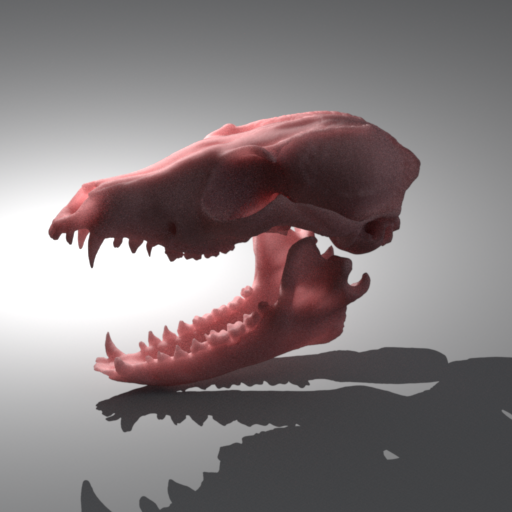
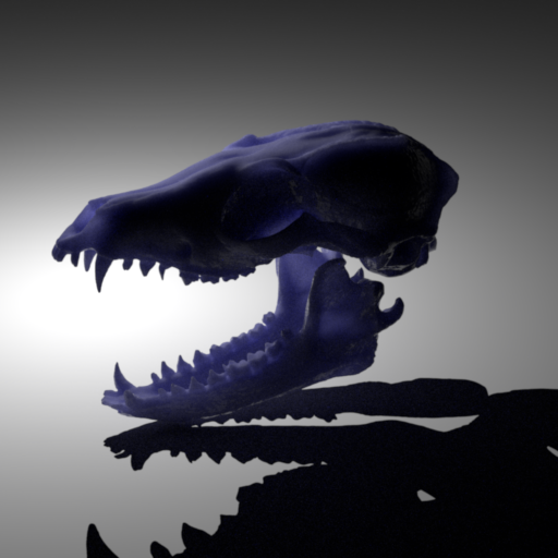
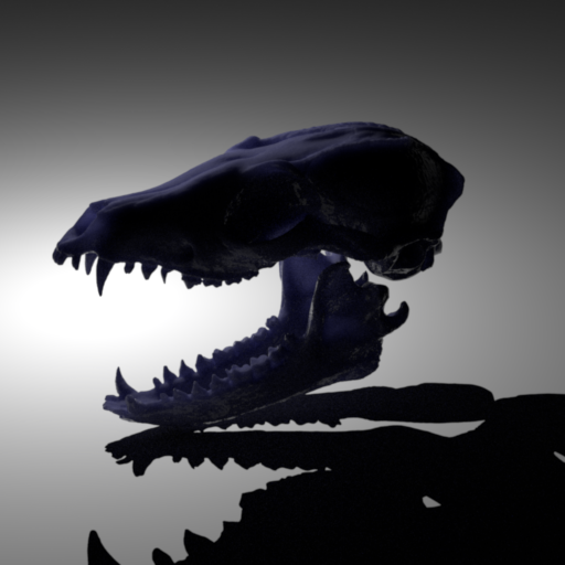
Comparison 0 - Enable / Disable SSS
First, we compare the render with and without subsurface scattering. One can easily recognize that the light skims though the thin parts, which is not the case of the diffuse-only version on the left.
- Mean free path: 0.2 m
- Albedo: 0.4,0.2,0.2
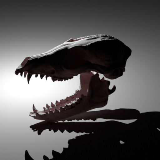
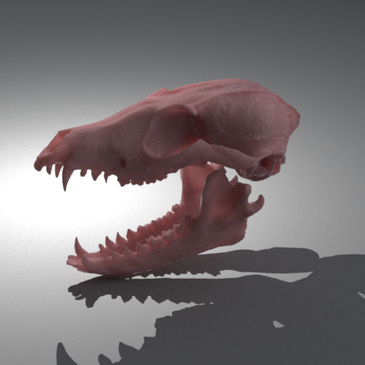
Comparison 1 - Basic setup
Basic setup with a point light. The energy distribution is slightly different between PBRT and Nori, but it can be seen nicely that the subsurface scattering has a similar effect around thin parts of the mesh.
- Mean free path: 0.2 m
- Albedo: 0.4,0.2,0.2
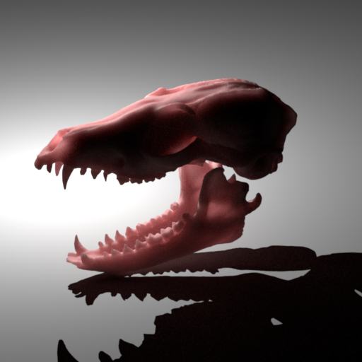
Comparison 2 - With Environment Light
When using an environment light emitter (see other feature) the discrepancy between the two approaches is larger. We suspect that this is caused by the additional materials added in the subsurface scattering case in PBRT. Our solution however looks plausible too and the importance sampling works well with very few exceptions. The subsurface scattering that is observable on the teeth and the nostrils still match the PBRT version.
- Mean free path: 0.2 m
- Albedo: 0.4,0.2,0.2
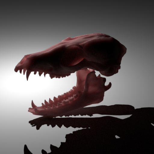
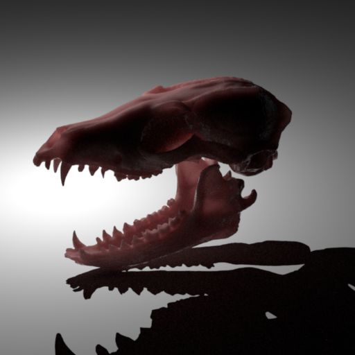
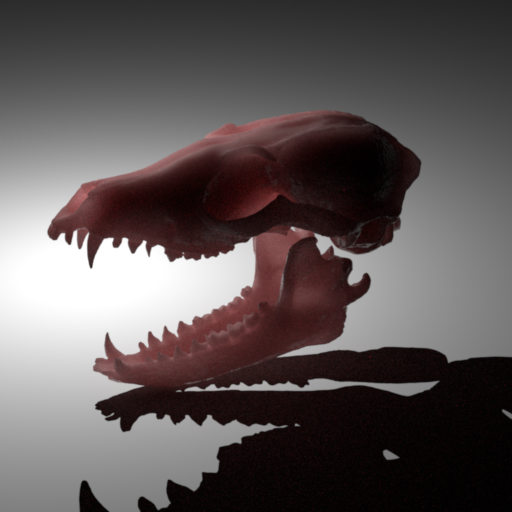
Comparison 3 - Different Albedos
In this validation, we inspect the effect of different albedo values. One can clearly observe that attenuating effect of lower albedo/diffuse radiance has on the subsurface scattering.
- Mean free path: 0.2 m
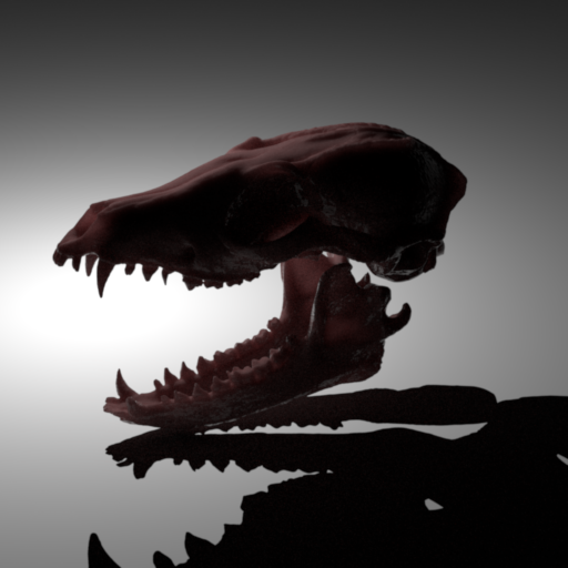
Comparison 3 - Different Mean Free Path Lengths
Here, we compare two different mean free path lengths in Nori. As expected, the longer the mean free path is, the more the light can travel through the object and the more prominent is the subsurface scattering.
- Albedo: 0.4,0.2,0.2
Code Coordinates
The implementation touches many places of our path tracer. In the following, we list the most important ones with a short description on what the code does:
bssrdf.h/bssrdf.cppHeader and code file with interfaces for the lookup table (BSSRDFTable), theBSSRDFbase class, theSeparableBSSRDFand theTabulatedBSSRDFwhich is a BSSRDF-implementation that allows to use a lookup table. Finally, this file contains the definition ofNoriBSSRDFandDirectionalSubsurface. The first one is made for interfacing with the path tracing components and simply invokes the functionality offered byTabulatedBSSRDF. The second one is a BSDF can be sampled to get an incoming direction for the subsurface scattering.interpolation.h/interpolation.cppAs described above, adapted from PBRT. This file implements Catmull-Rom interpolation to interpolate values in the lookup table.path_mis.cppTo accommodate for the added subsurface scattering, we changed the structure of path_mis to re-use the BSDF- and emitter sampling in multiple places. This has a great impact of the structure.- Other We also add an additional flags to the
BSDFQueryRecord,isTransmissionand two flags to theEmitter.h,isDiffuseandisSpecular. While theisSpecularcould also be evaluated over theBSDFQueryRecord.measurefield, this is a bit of a cleaner way to do it.