Data
Numerical Simulations
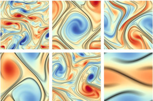
The following list contains a number of numerical data sets that we released for any use. If you use the data in your publications, please acknowledge the contributors by using the provided citation next to the download links. All data sets are provided in NetCDF format, the Amira format and the VTK format. The NetCDF format is highly recommended, as it contains many useful properties, such as the physical units and the parameters of the simulation (obstacles, viscosity, Reynolds number if available).2D Unsteady Fluid Simulation Ensemble for Machine Learning
 Example flows |
Regular grid:
Web browser access (2 GB/file)
File server access (2 GB/file)
Citation Ensemble simulation of 8,000 unsteady 2D flows with spatially-periodic boundary conditions. The simulation was done with Gerris flow solver and is carried out on a regular grid. The 8,000 flows are ordered from laminar configurations to turbulent configurations. The last column and row are left out, since they are the same as the first column and row. A detailed description of the data set can be found in Jakob et al.. Regular grid resolution (X x Y x T): 512 x 512 x 1001 Simulation domain: [0, 1] x [0, 1] x [0, 10] Reynolds Number range: [1, 4096] Kinematic viscosity range: [1e-5, 1e-4] |
2D Unsteady Cylinder Flow with von Karman Vortex Street
 Line integral convolution 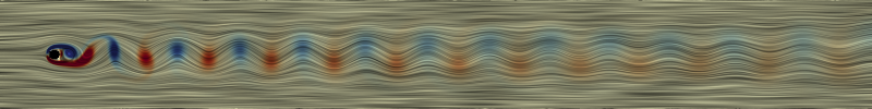 Vorticity 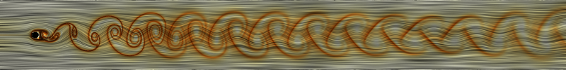 Finite-time Lyapunov exponent (backward) |
Regular grid:
NetCDF (440 MB)
Amira (460 MB)
VTK (448 MB)
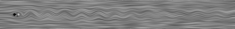
Unstructured grid: VTK (4.83 GB) Citation Simulation of a viscous 2D flow around a cylinder. The fluid was injected to the left of a channel bounded by solid walls with a slip boundary condition. The simulation was done with Gerris flow solver and was resampled onto a regular grid. In the original simulation, the unstructured grid was adaptively discretized based on the vorticity. Over the course of the simulation, the characteristic von-Karman vortex street is forming. The image on the side shows a later time step, in which the street is fully formed. The vortices move with almost constant speed, except directly in the wake of the obstacle, where they accelerate. Regular grid resolution (X x Y x T): 640 x 80 x 1501 Simulation domain: [-0.5, 7.5] x [-0.5, 0.5] x [0, 15] Reynolds Number: 160 Kinematic viscosity: 0.00078125 Obstacle at (0,0) with radius: 0.0625 |
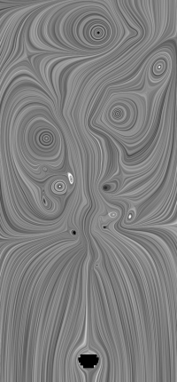
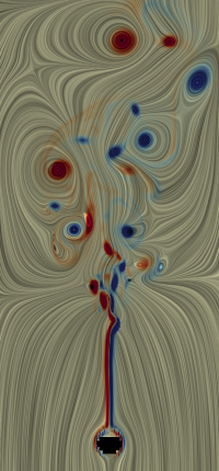
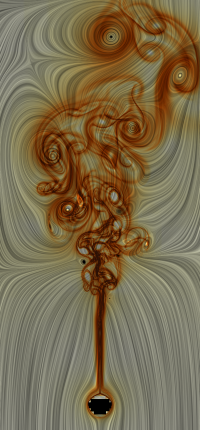
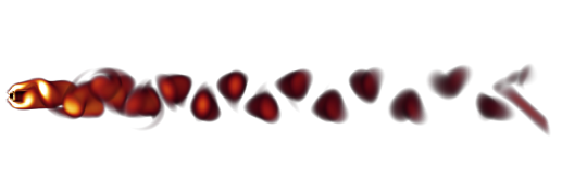
2D Unsteady Heated Cylinder with Boussinesq Approximation
|
Regular grid:
NetCDF (903 MB)
Amira (922 MB)
VTK (908 MB)
Unstructured grid: VTK (1.68 GB) Citation Simulation of a 2D flow generated by a heated cylinder. To solve the buoyancy problem, the Boussinesq approximation is used. The simulation was done with Gerris flow solver and was resampled onto a regular grid. The turbulent plume contains numerous small vortices that in part rotate around each other. Grid resolution (X x Y x T): 150 x 450 x 2001 Simulation domain: [-0.5, 0.5] x [-0.5, 2.5] x [0, 20] Obstacle at (0,-0.15) with radius: 0.0625 |
2D Unsteady Cylinder Flow Around Corners
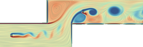 Vorticity 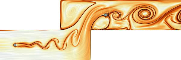 Finite-time Lyapunov exponent (backward) |
Regular grid:
NetCDF (409 MB)
Amira (414 MB)
VTK (412 MB)
Unstructured grid: VTK (518 MB) Citation Simulation of a viscous 2D flow around two cylinders. The fluid was injected to the left of a channel bounded by solid walls with a slip boundary condition. The simulation was done with Gerris flow solver and was resampled onto a regular grid. In the original simulation, the unstructured grid was adaptively discretized based on the vorticity. Initially, a vortex street forms behind the first obstacle, which then flows around two corners. Behind each corner, a standing vortex forms. The latter one blocks half of the flow to the second obstacle, creating a one-sided vortex street. Regular grid resolution (X x Y x T): 450 x 150 x 1501 Simulation domain: [-0.5, 5.5] x [-0.5, 1.5] x [0, 15] Reynolds Number: 160 Kinematic viscosity: 0.00078125 Obstacles at (0,0) and (3,1) both with radius: 0.0625 |
3D Steady Cloud-topped Boundary Layer
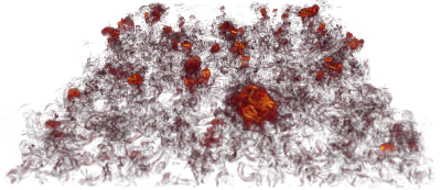 Vorticity |
Regular grid:
NetCDF (201 MB)
Amira (202 MB)
VTK (202 MB)
Citation This data set contains a cloud resolving boundary layer simulation that was simulated with the UCLA-LES model. In the domain, you will find a number of rising cumulus clouds. The data set is kindly provided by the German Climate Computing Center (DKRZ) and the Max Planck Insitute for Meteorology (MPI-M), and was simulated in the HD(CP)2 project. The simulation uses double-periodic boundary conditions, a homogeneous surface forcing, and takes its large-scale information from the COSMO-DE simulation model. Regular grid resolution (X x Y x Z): 384 x 384 x 130 Simulation domain: [0, 10] x [0, 10] x [0, 3.2] |
3D Unsteady Half Cylinder Ensemble
 Vorticity for Reynolds number: 160 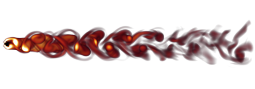 Vorticity for Reynolds number: 320 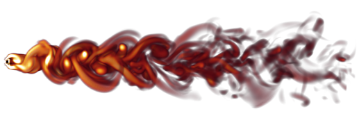 Vorticity for Reynolds number: 640 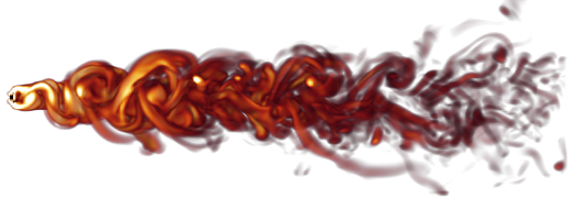 Vorticity for Reynolds number: 6400 |
Re = 160
Regular grid: NetCDF (17.7 GB) Amira (18.7 GB) VTK (17.9 GB) Unstructured grid: VTK (1.2 GB) Re = 320 Regular grid: NetCDF (17.6 GB) Amira (18.6 GB) VTK (17.8. GB) Unstructured grid: VTK (1.4 GB) Re = 640 Regular grid: NetCDF (17.6 GB) Amira (18.6 GB) VTK (17.9 GB) Unstructured grid: VTK (1.5 GB) Re = 6400 Regular grid: NetCDF (17.6. GB) Amira (18.6 GB) VTK (17.9 GB) Unstructured grid: VTK (1.9 GB) Citation Small ensemble of numerical simulations of an incompressible 3D flow around a half cylinder. Each ensemble member was simulated with a different Reynolds number (Re). The simulations were done with Gerris flow solver and were resampled onto a regular grid. In the original simulation, the unstructured grid was adaptively discretized based on the vorticity. This flow might be useful for ensemble visualization techniques or for tests on flows with varying degree of turbulence. Regular grid resolution (X x Y x Z x T): 640 x 240 x 80 x 151 Simulation domain: [-0.5, 7.5] x [-1.5, 1.5] x [-0.5, 0.5] x [0, 2] Reynolds Numbers: 160, 320, 640, 6400 |
3D Unsteady Research Vessel Tangaroa
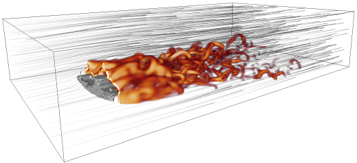 Vorticity in wake of the ship |
Regular grid:
NetCDF (12.5 GB)
Amira (13.1 GB)
VTK (12.7 GB)
Unstructured grid: VTK (2.1 GB) Citation Simulation of an incompressible 3D flow around a CAD model of the research vessel Tangaroa. The simulation was done with Gerris flow solver and a region of interest was resampled onto a regular grid. This is one of the example simulations of Gerris flow solver. In the original simulation, the unstructured grid was adaptively discretized based on the vorticity. Regular grid resolution (X x Y x Z x T): 300 x 180 x 120 x 201 Simulation domain: [-0.35, 0.65] x [-0.3, 0.3] x [-0.5, -0.3] x [0, 2] |
Analytic Vector Fields
It can come in very handy to test algorithms on analytic vector fields. For each analytic data set, the formular of the vector field itself and the first-order partial derivatives are provided in C++, Matlab and Python. For ease of use and testing, the vector fields are sampled onto regular grids, as well.2D Unsteady Double Gyre
 LIC with vorticity 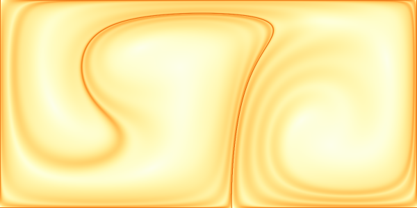 Finite-time Lyapunov exponent |
NetCDF (108 MB)
Amira (113 MB)
VTK (117 MB)
C++ code Matlab code Python code Citation The double gyre is a periodic time-dependent vector field, in which a separating boundary oscillates horizontally between two oppositely rotating vortices. The flow was introduced by Shadden et al. and became the prime benchmark for finite-time Lyapunov exponents. The analytic formular has several parameters that steer magnitude (A), oscillation frequency (omega) and oscillation amplitude (eps). The resampled versions use the standard parameters listed below. The flow is also spatially periodic, which allows variations that contain saddles in the interior of the domain, such as the quad gyre with [0,2] x [-1,1] x [0,10]. Grid resolution (X x Y x T): 256 x 128 x 512 Space-time Domain: [0, 2] x [0, 1] x [0, 10] Standard parameters: A = 0.1, omega = pi/5, eps = 0.25 |
2D Unsteady Beads Problem
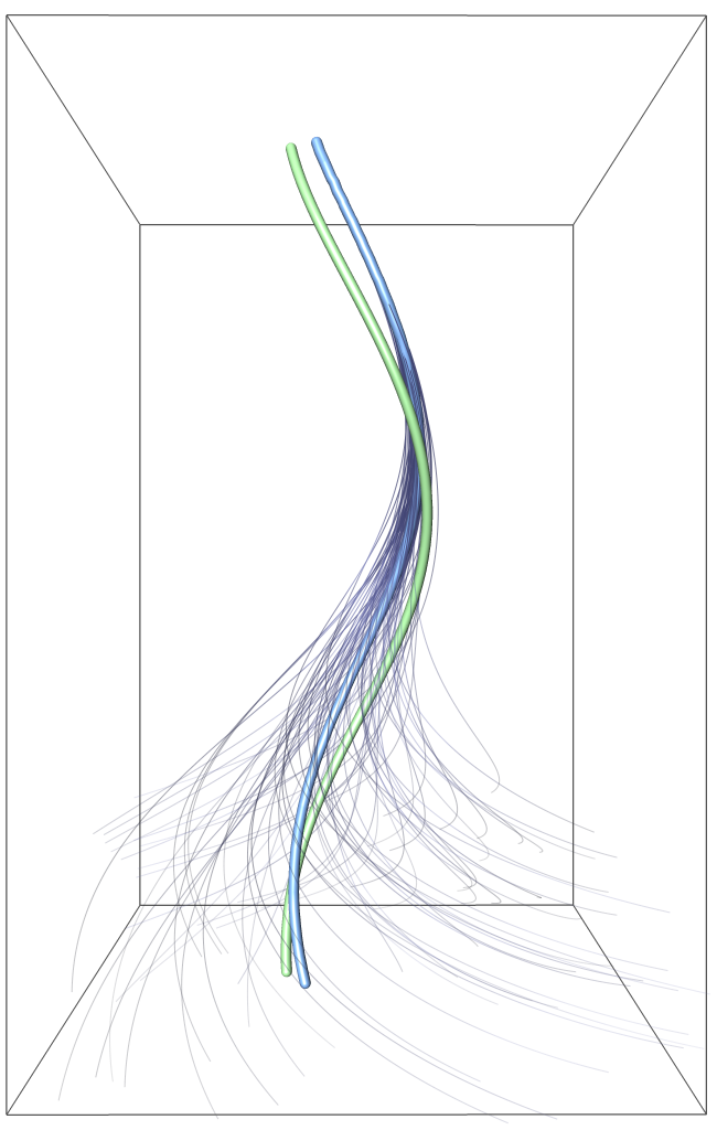 Vortex corelines in the Beads problem, image from here |
NetCDF (775 KB)
Amira (13.8 MB)
VTK (837 KB)
C++ code Matlab code Python code Citation Wiebel et al. studied particle motion in a rotating petri-dish, which proved to become a challenging benchmark for vortex coreline extraction, since the vortex center is moving on a circular path, which is not covered by Galilean invariant vortex extractors. An analytic approximation to this flow was for instance given by Weinkauf and Theisel, which is provided here. The image on the side shows pathlines that are attracted to the true coreline (blue), compared to a Galilean invariant coreline extraction (green). Grid resolution (X x Y x T): 128 x 128 x 512 Simulation domain: [-2, 2] x [-2, 2] x [0, 2pi] |
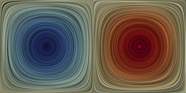
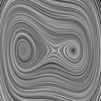
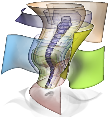
2D Unsteady Four Rotating Centers
|
NetCDF (54 MB)
Amira (56.3 MB)
VTK (57.5 MB)
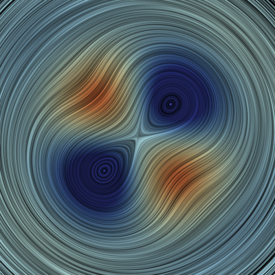
C++ code Matlab code Python code Citation This analytic data set contains four vortices. The flow is made unsteady by performing a uniform reference frame rotation. User parameters are a scaling factor of the magnitude (scale) and the speed of the reference frame rotation (al_t). The vortex centers are positioned at t=0 at ± 2^(-1/2). The construction of the data set is described here in Section 7.2. This data set is a good benchmark for reference frame invariant flow feature extraction, since simple Galilean invariance is not enough. Grid resolution (X x Y x T): 128 x 128 x 512 Space-time domain: [-2, 2] x [-2, 2] x [0, 2pi] Standard parameters: scale = 1, al_t = 1 |
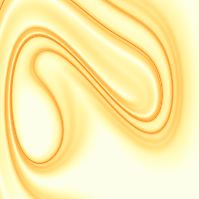
2D Unsteady Forced-Damped Duffing Oscillator
|
NetCDF (30.1 MB)
Amira (31 MB)
VTK (29.9 MB)
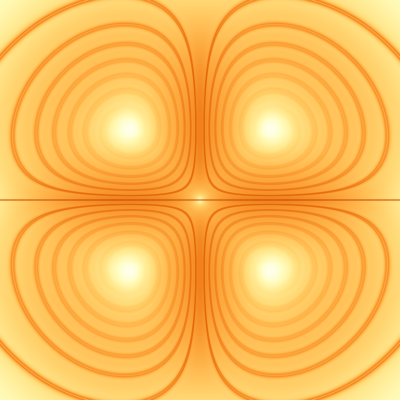
C++ code Matlab code Python code Citation This analytic vector field describes the phase space of a duffing oscillator with forcing and damping. For the standard parameters, the vector fields contains a saddle-type periodic orbit. Grid resolution (X x Y x T): 128 x 128 x 512 Space-time domain: [-2, 2] x [-2, 2] x [0, 4] Standard parameters: alpha = -0.25, beta = 0.4 |
2D Unsteady Cylinder Flow (Synthetic)
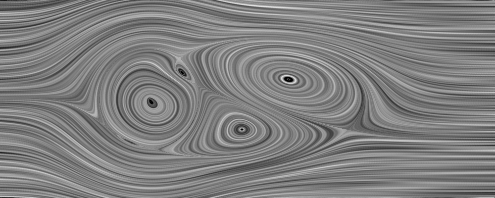 Line integral convolution |
NetCDF (311 MB)
Amira (317 MB)
VTK (313 MB)
Citation This synthetic vector field represents a simple model of a von-Karman vortex street generation and was constructed by Jung, Tel and Ziemniak as co-gradient to a stream function. The obstacle is positioned at (0,0) and has a radius=1. In the LIC image on the side, the flow in the interior of the obstacle has not been set to zero. Note that only two vortices are present at the same time. In the files above, we sampled four periods onto a regular grid. Grid resolution (X x Y x T): 450 x 200 x 500 Spatial domain: [-3, 7] x [-2, 2] x [1.107, 5.535] |
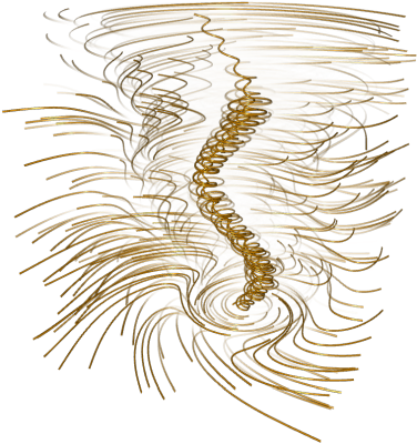
3D Steady Tornado (Synthetic)
|
NetCDF (16.9 MB)
Amira (17.7 MB)
VTK (17.0 MB)
Citation This synthetic model of a tornado was created by Roger Crawfis and was made available as C code here. We scaled the flow to a larger domain and sampled it onto a regular grid. If higher resolutions are required, simply run the C code. Grid resolution (X x Y x Z): 128 x 128 x 128 Spatial domain: [-10, 10] x [-10, 10] x [-10, 10] |
More Scientific Data Sets
Haven't found the right data set yet? The following list contains a number of pointers.Point Data
Unsteady 3D Dark Sky Simulation - VisContest 2015
Unsteady 3D Ensemble of Salt Dissolving in Water - VisContest 2016
Unsteady 3D Cosmology Simulation - VisContest 2019
Unsteady 3D Ensemble of Salt Dissolving in Water - VisContest 2016
Unsteady 3D Cosmology Simulation - VisContest 2019
Scalar Fields
Steady 3D High Resolution microCT Scans - University of Zurich
Steady 3D Scan of Christmas Present, Stag Beetle and Christmas Tree - TU Vienna
Unsteady 3D Satellite Data of Volcanic Eruptions - VisContest 2014
Steady 3D Scan of Christmas Present, Stag Beetle and Christmas Tree - TU Vienna
Unsteady 3D Satellite Data of Volcanic Eruptions - VisContest 2014
Vector Fields
Unsteady 2D Cylinder Flow - by Tino Weinkauf
Unsteady 3D Flow around Square Cylinder - by Tino Weinkauf
Unsteady 3D Fields of Hurriance Isabel - VisContest 2004
Unsteady 3D Fields of Earthquake - VisContest 2006
Unsteady 3D Ensemble of Centrifugal Pump - VisContest 2011
Unsteady 3D Fields of Clouds over Germany - VisContest 2017
Unsteady 3D Ensemble of Asteroid Impacts in Deep Water Oceans - VisContest 2018
Unsteady 3D Fields of High Resolution Turbulence - John Hopkins Turbulence Database
Unsteady 3D Fields of Numerical Weather Forecasting - European Center For Medium Range Weather Forecasting (ECMWF)
How Can I Read the Data Sets?
In general, NetCDF is the recommend format. Readers exist for almost all languages (C++, Matlab, Python, ...). If you write C++ code and do not want to depend on other libraries, have a look at the Amira reader of Tino Weinkauf here. If you are compiling with VTK anyway, you can use the VTK readers. ParaView should have no problems to open the VTK files.Let me know if you need help to open the data. We can learn from it and provide more information on this website to also help the next person.